Transfer learning and pre-training schemas for both NLP and Computer Vision have gained a lot of attention in the last months. Research showed that carefully designed unsupervised/self-supervised training can produce high quality base models and embeddings that greatly decrease the amount of data needed to obtain good classification models downstream. This approach becomes more and more important as the companies collect a lot of data from which only a fraction can be labelled by humans - either due to large cost of labelling process or due to some time constraints.
Here I explore SimCLR pre-training framework proposed by Google in this arxiv paper. I will explain the SimCLR and its contrastive loss function step by step, starting from naive implementation in PyTorch, followed by faster, vectorized one. Then I will show how to use SimCLR’s pre-training routine to first build image embeddings using EfficientNet network architecture and finally I will show how to build a classifier on top of it.
TL;DR
This post covers:
- understanding the SimCLR framework with code samples in PyTorch
- from scratch explanation & implementation of SimCLR’s loss function (NT-Xent) in PyTorch
- pre-training image embeddings using EfficientNet architecture
- training classifier by using transfer learning from the pre-trained embeddings
Understanding SimCLR framework
In general, SimCLR is a simple framework for contrastive learning of visual representations. It’s not any new framework for deep learning, it’s a set of fixed steps that one should follow in order to train image embeddings of good quality. I drew a schema which explains the flow and the whole representation learning process (click to zoom).

The flow is as follows (from left to right):
- Take an input image
- Prepare 2 random augmentations on the image, including: rotations, hue/saturation/brightness changes, zooming, cropping, etc. The range of augmentations as well as analysis which ones work best are discussed in detail in the paper.
- Run a deep neural network (preferably convolutional one, like ResNet50) to obtain image representations (embeddings) for those augmented images.
- Run a small fully connected linear neural network to project embeddings into another vector space.
- Calculate contrastive loss and run backpropagation through both networks. Contrastive loss decreases when projections coming from the same image are similar. The similarity between projections can be arbitrary, here I will use cosine similarity, same as in the paper.
Contrastive loss function
Theory behind contrastive loss function
One can reason about contrastive loss function form two angles:
- Contrastive loss decreases when projections of augmented images coming from the same input image are similar.
- For two augmented images: (i), (j) (coming from the same input image - I will call them “positive” pair later on), the contrastive loss for (i) tries to identify (j) among other images (“negative” examples) that are in the same batch .
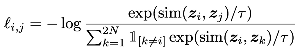
Formal definition of the loss for pair of positive examples (i) and (j) defined as:

The final loss is an arithmetic mean of the losses for all positive pairs in the batch:

(keep in mind that the indexing in l(2k-1, 2k) + l(2k, 2k-1) is purely dependent on how you implement the loss - I find it easier to understand when I reason about them as l(i,j) + l(j,i)).
Contrastive loss function - implementation in PyTorch, ELI5 version
It’s much easier to implement the loss function without vectorization first and then follow up with the vectorization phase.
import torch
from torch import nn
import torch.nn.functional as F
class ContrastiveLossELI5(nn.Module):
    def __init__(self, batch_size, temperature=0.5, verbose=True):
        super().__init__()
        self.batch_size = batch_size
        self.register_buffer("temperature", torch.tensor(temperature))
        self.verbose = verbose

    def forward(self, emb_i, emb_j):
        """
        emb_i and emb_j are batches of embeddings, where corresponding indices are pairs
        z_i, z_j as per SimCLR paper
        """
        z_i = F.normalize(emb_i, dim=1)
        z_j = F.normalize(emb_j, dim=1)

        representations = torch.cat([z_i, z_j], dim=0)
        similarity_matrix = F.cosine_similarity(representations.unsqueeze(1), representations.unsqueeze(0), dim=2)
        if self.verbose: print("Similarity matrix\n", similarity_matrix, "\n")

        def l_ij(i, j):
            z_i_, z_j_ = representations[i], representations[j]
            sim_i_j = similarity_matrix[i, j]
            if self.verbose: print(f"sim({i}, {j})={sim_i_j}")

            numerator = torch.exp(sim_i_j / self.temperature)
            one_for_not_i = torch.ones((2 * self.batch_size, )).to(emb_i.device).scatter_(0, torch.tensor([i]), 0.0)
            if self.verbose: print(f"1{{k!={i}}}",one_for_not_i)

            denominator = torch.sum(
                one_for_not_i * torch.exp(similarity_matrix[i, :] / self.temperature)
            )
            if self.verbose: print("Denominator", denominator)

            loss_ij = -torch.log(numerator / denominator)
            if self.verbose: print(f"loss({i},{j})={loss_ij}\n")

            return loss_ij.squeeze(0)

        N = self.batch_size
        loss = 0.0
        for k in range(0, N):
            loss += l_ij(k, k + N) + l_ij(k + N, k)
        return 1.0 / (2*N) * loss
Explanation
Contrastive loss needs to know the batch size and temperature (scaling) parameter. You can find details about setting the optimal temperature parameter in the paper.
My implementation of the forward of the contrastive loss takes two parameters. First one will be a batch projection of images after first augmentation, the second will be a batch projection of images after second augmentation.
Projections needs to be normalized first, hence:
z_i = F.normalize(emb_i, dim=1)
z_j = F.normalize(emb_j, dim=1)
All representations are concatenated together in order to efficiently calculate cosine similarities between each image pair.
representations = torch.cat([z_i, z_j], dim=0)
similarity_matrix = F.cosine_similarity(representations.unsqueeze(1), representations.unsqueeze(0), dim=2)
Next is the naive implementation of l(i,j) for clarity and easiness of understanding. The code bellow almost directly implements the equation:
def l_ij(i, j):
    z_i_, z_j_ = representations[i], representations[j]
    sim_i_j = similarity_matrix[i, j]
    numerator = torch.exp(sim_i_j / self.temperature)
    one_for_not_i = torch.ones((2 * self.batch_size, )).to(emb_i.device).scatter_(0, torch.tensor([i]), 0.0)
    denominator = torch.sum(
        one_for_not_i * torch.exp(similarity_matrix[i, :] / self.temperature)
    )

    loss_ij = -torch.log(numerator / denominator)
    return loss_ij.squeeze(0)
Then, the final loss for the batch is computed as an arithmetic mean of all combinations of positive examples:
N = self.batch_size
loss = 0.0
for k in range(0, N):
    loss += l_ij(k, k + N) + l_ij(k + N, k)
return 1.0 / (2*N) * loss
Now, let’s run it with verbose mode to see what’s inside.
I = torch.tensor([[1.0, 2.0], [3.0, -2.0], [1.0, 5.0]])
J = torch.tensor([[1.0, 0.75], [2.8, -1.75], [1.0, 4.7]])
loss_eli5 = ContrastiveLossELI5(batch_size=3, temperature=1.0, verbose=True)
loss_eli5(I, J)
Similarity matrix
    tensor([[ 1.0000, -0.1240,  0.9648,  0.8944, -0.0948,  0.9679],
        [-0.1240,  1.0000, -0.3807,  0.3328,  0.9996, -0.3694],
        [ 0.9648, -0.3807,  1.0000,  0.7452, -0.3534,  0.9999],
        [ 0.8944,  0.3328,  0.7452,  1.0000,  0.3604,  0.7533],
        [-0.0948,  0.9996, -0.3534,  0.3604,  1.0000, -0.3419],
        [ 0.9679, -0.3694,  0.9999,  0.7533, -0.3419,  1.0000]])

sim(0, 3)=0.8944272398948669
1{k!=0} tensor([0., 1., 1., 1., 1., 1.])
Denominator tensor(9.4954)
loss(0,3)=1.3563847541809082

sim(3, 0)=0.8944272398948669
1{k!=3} tensor([1., 1., 1., 0., 1., 1.])
Denominator tensor(9.5058)
loss(3,0)=1.357473373413086

sim(1, 4)=0.9995677471160889
1{k!=1} tensor([1., 0., 1., 1., 1., 1.])
Denominator tensor(6.3699)
loss(1,4)=0.8520082831382751

sim(4, 1)=0.9995677471160889
1{k!=4} tensor([1., 1., 1., 1., 0., 1.])
Denominator tensor(6.4733)
loss(4,1)=0.8681114912033081

sim(2, 5)=0.9999250769615173
1{k!=2} tensor([1., 1., 0., 1., 1., 1.])
Denominator tensor(8.8348)
loss(2,5)=1.1787779331207275

sim(5, 2)=0.9999250769615173
1{k!=5} tensor([1., 1., 1., 1., 1., 0.])
Denominator tensor(8.8762)
loss(5,2)=1.1834462881088257

tensor(1.1327)
A few things happened there, but by going back and forward between the verbose logs and the equation, everything should become clear.
The indexing jumps by batch size (first l(0,3), l(3,0) then l(1,4), l(4,1) because of the way the similarity matrix was constructed. First row of the similarity_matrix is:
[ 1.0000, -0.1240, 0.9648, 0.8944, -0.0948, 0.9679]
Remember the input:
I = torch.tensor([[1.0, 2.0], [3.0, -2.0], [1.0, 5.0]])
J = torch.tensor([[1.0, 0.75], [2.8, -1.75], [1.0, 4.7]])
Now:
1.0000 is the cosine similarity between I[0] and I[0] ([1.0, 2.0] and [1.0, 2.0])
-0.1240 is the cosine similarity between I[0] and I[1] ([1.0, 2.0] and [3.0, -2.0])
-0.0948 is the cosine similarity between I[0] and J[2] ([1.0, 2.0] and [2.8, -1.75])
… and so on.
Let’s see if the loss decreases if the similarity between first image projection increases:
I = torch.tensor([[1.0, 2.0], [3.0, -2.0], [1.0, 5.0]])
J = torch.tensor([[1.0, 0.75], [2.8, -1.75], [1.0, 4.7]])
J = torch.tensor([[1.0, 1.75], [2.8, -1.75], [1.0, 4.7]]) # note the change
ContrastiveLossELI5(3, 1.0, verbose=False)(I, J)
tensor(1.0996)
Indeed the loss decreases! Now I will follow up with the vectorized implementation.
Contrastive loss function - implementation in PyTorch, vectorized version
Performance of naive implementation is really poor (mostly due to manual loop), see the results:
contrastive_loss_eli5 = ContrastiveLossELI5(3, 1.0, verbose=False)
I = torch.tensor([[1.0, 2.0], [3.0, -2.0], [1.0, 5.0]], requires_grad=True)
J = torch.tensor([[1.0, 0.75], [2.8, -1.75], [1.0, 4.7]], requires_grad=True)
%%timeit
contrastive_loss_eli5(I, J)
838 µs ± 23.8 µs per loop (mean ± std. dev. of 7 runs, 1000 loops each)
Once I understood the internals of the loss, it’s easy to vectorize it and remove the manual loop:
class ContrastiveLoss(nn.Module):
    def __init__(self, batch_size, temperature=0.5):
        super().__init__()
        self.batch_size = batch_size
        self.register_buffer("temperature", torch.tensor(temperature))
        self.register_buffer("negatives_mask", (~torch.eye(batch_size * 2, batch_size * 2, dtype=bool)).float())

    def forward(self, emb_i, emb_j):
        """
        emb_i and emb_j are batches of embeddings, where corresponding indices are pairs
        z_i, z_j as per SimCLR paper
        """
        z_i = F.normalize(emb_i, dim=1)
        z_j = F.normalize(emb_j, dim=1)

        representations = torch.cat([z_i, z_j], dim=0)
        similarity_matrix = F.cosine_similarity(representations.unsqueeze(1), representations.unsqueeze(0), dim=2)

        sim_ij = torch.diag(similarity_matrix, self.batch_size)
        sim_ji = torch.diag(similarity_matrix, -self.batch_size)
        positives = torch.cat([sim_ij, sim_ji], dim=0)

        nominator = torch.exp(positives / self.temperature)
        denominator = self.negatives_mask * torch.exp(similarity_matrix / self.temperature)

        loss_partial = -torch.log(nominator / torch.sum(denominator, dim=1))
        loss = torch.sum(loss_partial) / (2 * self.batch_size)
        return loss
contrastive_loss = ContrastiveLoss(3, 1.0)
contrastive_loss(I, J).item() - contrastive_loss_eli5(I, J).item()
0.0
The difference should be zero or close to zero (< 1e-6 due to fp arithmetics). Performance comparison:
I = torch.tensor([[1.0, 2.0], [3.0, -2.0], [1.0, 5.0]], requires_grad=True)
J = torch.tensor([[1.0, 0.75], [2.8, -1.75], [1.0, 4.7]], requires_grad=True)
%%timeit
contrastive_loss_eli5(I, J)
918 µs ± 60.2 µs per loop (mean ± std. dev. of 7 runs, 1000 loops each)
%%timeit
contrastive_loss(I, J)
272 µs ± 9.18 µs per loop (mean ± std. dev. of 7 runs, 1000 loops each)
Almost 4x improvement, it works.
Pre-training image embeddings using SimCLR with EfficientNet
Once the loss function is established and understood it’s time to make a good use of it. I will pre-train image embeddings using EfficientNet architecture, following the SimCLR framework. For convenience, I’ve implemented a few utility functions and classes that I will explain briefly below. The training code is structured using PyTorch-Lightning.
I will use a great EfficientNet [https://arxiv.org/abs/1905.11946] implementation by Luke Melas-Kyriazi from GitHub, already pre-trained on ImageNet (transfer learning inception!). The dataset I choose is STL10 (from torchvision) as it contains both training and unlabeled splits for unsupervised / self-supervised learning tasks.
My goal here is to demonstrate the whole SimCLR flow from start to the end. I had no intent to reach new SOTA with the presented configuration.
Utility functions for image augmentations
Training with SimCLR produces good image embeddings that are not affected by image transformations - this is because during training, various data augmentations are done to force the network to understand the contents of the images regardless of i.e color of the image or the position where the object in the image is placed. SimCLR’s authors say that composition of data augmentations plays a critical role in defining effective predictive tasks and also contrastive learning needs stronger data augmentation than supervised learning. To sum this up: when pre-training the image embeddings it’s good to make this task difficult for the network to learn by strongly augmenting the images in order to generalize better afterwards.
I strongly advise to read the SimCLR’s paper and it’s appendix as they did ablation studies on which data augmentations bring the best effects on the embeddings.
To keep this blog-post simple to go through, I will mostly use built-in Torchvision’s data augmentations , with one additional one - random resized rotation.
def random_rotate(image):
    if random.random() > 0.5:
        return tvf.rotate(image, angle=random.choice((0, 90, 180, 270)))
    return image
class ResizedRotation():
    def __init__(self, angle, output_size=(96, 96)):
        self.angle = angle
        self.output_size = output_size

    def angle_to_rad(self, ang): return np.pi * ang / 180.0

    def __call__(self, image):
        w, h = image.size
        new_h = int(np.abs(w * np.sin(self.angle_to_rad(90 - self.angle))) + np.abs(h * np.sin(self.angle_to_rad(self.angle))))
        new_w = int(np.abs(h * np.sin(self.angle_to_rad(90 - self.angle))) + np.abs(w * np.sin(self.angle_to_rad(self.angle))))
        img = tvf.resize(image, (new_w, new_h))
        img = tvf.rotate(img, self.angle)
        img = tvf.center_crop(img, self.output_size)
        return img
class WrapWithRandomParams():
    def __init__(self, constructor, ranges):
        self.constructor = constructor
        self.ranges = ranges

    def __call__(self, image):
        randoms = [float(np.random.uniform(low, high)) for _, (low, high) in zip(range(len(self.ranges)), self.ranges)]
        return self.constructor(*randoms)(image)
from torchvision.datasets import STL10
import torchvision.transforms.functional as tvf
from torchvision import transforms
import numpy as np
A brief look on the transformation results:
stl10_unlabeled = STL10(".", split="unlabeled", download=True)
idx = 123
random_resized_rotation = WrapWithRandomParams(lambda angle: ResizedRotation(angle), [(0.0, 360.0)])
random_resized_rotation(tvf.resize(stl10_unlabeled[idx][0], (96, 96)))

Automatic data augmentation wrapper
Here I’ve also implemented a utility dataset wrapper that automatically applies random data augmentations every time when the image is retrieved. It can be easily used with any image dataset as long as it follows the simple interface of returning tuple with (PIL Image, anything). This wrapper can be set to return a deterministic transformation with the debug flag set to True. Note that there is a preprocess step that applies ImageNet-originated data standardization as I’m using already pre-trained EfficientNet.
from torch.utils.data import Dataset, DataLoader, SubsetRandomSampler, SequentialSampler
import random
class PretrainingDatasetWrapper(Dataset):
    def __init__(self, ds: Dataset, target_size=(96, 96), debug=False):
        super().__init__()
        self.ds = ds
        self.debug = debug
        self.target_size = target_size
        if debug:
            print("DATASET IN DEBUG MODE")

        # I will be using network pre-trained on ImageNet first, which uses this normalization.
        # Remove this, if you're training from scratch or apply different transformations accordingly
        self.preprocess = transforms.Compose([
                transforms.ToTensor(),
                transforms.Normalize(mean=[0.485, 0.456, 0.406], std=[0.229, 0.224, 0.225]),
        ])

        random_resized_rotation = WrapWithRandomParams(lambda angle: ResizedRotation(angle, target_size), [(0.0, 360.0)])
        self.randomize = transforms.Compose([
            transforms.RandomResizedCrop(target_size, scale=(1/3, 1.0), ratio=(0.3, 2.0)),
            transforms.RandomChoice([
                transforms.RandomHorizontalFlip(p=0.5),
                transforms.Lambda(random_rotate)
            ]),
            transforms.RandomApply([
                random_resized_rotation
            ], p=0.33),
            transforms.RandomApply([
                transforms.ColorJitter(brightness=0.5, contrast=0.5, saturation=0.5, hue=0.2)
            ], p=0.8),
            transforms.RandomGrayscale(p=0.2)
        ])

    def __len__(self): return len(self.ds)

    def __getitem_internal__(self, idx, preprocess=True):
        this_image_raw, _ = self.ds[idx]

        if self.debug:
            random.seed(idx)
            t1 = self.randomize(this_image_raw)
            random.seed(idx + 1)
            t2 = self.randomize(this_image_raw)
        else:
            t1 = self.randomize(this_image_raw)
            t2 = self.randomize(this_image_raw)

        if preprocess:
            t1 = self.preprocess(t1)
            t2 = self.preprocess(t2)
        else:
            t1 = transforms.ToTensor()(t1)
            t2 = transforms.ToTensor()(t2)

        return (t1, t2), torch.tensor(0)

    def __getitem__(self, idx):
        return self.__getitem_internal__(idx, True)

    def raw(self, idx):
        return self.__getitem_internal__(idx, False)
ds = PretrainingDatasetWrapper(stl10_unlabeled, debug=False)
tvf.to_pil_image(ds[idx][0][0])

tvf.to_pil_image(ds[idx][0][1])

tvf.to_pil_image(ds.raw(idx)[0][1])

tvf.to_pil_image(ds.raw(idx)[0][0])

SimCLR neural network for embeddings
Here I define the ImageEmbedding neural network which is based on EfficientNet-b0 architecture. I swap out the last layer of pre-trained EfficientNet with identity function and add projection for image embeddings on top of it (following the SimCLR paper) with Linear-ReLU-Linear layers. It was shown in the paper that the non-linear projection head (i.e Linear-ReLU-Linear) improves the quality of the embeddings.
from efficientnet_pytorch import EfficientNet
class ImageEmbedding(nn.Module):
    class Identity(nn.Module):
        def __init__(self): super().__init__()

        def forward(self, x):
            return x


    def __init__(self, embedding_size=1024):
        super().__init__()

        base_model = EfficientNet.from_pretrained("efficientnet-b0")
        internal_embedding_size = base_model._fc.in_features
        base_model._fc = ImageEmbedding.Identity()

        self.embedding = base_model

        self.projection = nn.Sequential(
            nn.Linear(in_features=internal_embedding_size, out_features=embedding_size),
            nn.ReLU(),
            nn.Linear(in_features=embedding_size, out_features=embedding_size)
        )

    def calculate_embedding(self, image):
        return self.embedding(image)

    def forward(self, X):
        image = X
        embedding = self.calculate_embedding(image)
        projection = self.projection(embedding)
        return embedding, projection
Next is the implementation of PyTorch-Lightning-based training module that orchestrates everything together:
- hyper-parameters handling
- SimCLR ImageEmbedding network
- STL10 dataset
- optimizer
- forward step
As the PretrainingDatasetWrapper I’ve implemented returns tuple of: (Image1, Image2), dummy class, the forward step for this module is straightforward - it needs to produce two batches of embeddings and calculate contrastive loss function:
(X, Y), y = batch
embX, projectionX = self.forward(X)
embY, projectionY = self.forward(Y)
loss = self.loss(projectionX, projectionY)
from torch.multiprocessing import cpu_count
from torch.optim import RMSprop
import pytorch_lightning as pl
class ImageEmbeddingModule(pl.LightningModule):
    def __init__(self, hparams):
        hparams = Namespace(**hparams) if isinstance(hparams, dict) else hparams
        super().__init__()
        self.hparams = hparams
        self.model = ImageEmbedding()
        self.loss = ContrastiveLoss(hparams.batch_size)

    def total_steps(self):
        return len(self.train_dataloader()) // self.hparams.epochs

    def train_dataloader(self):
        return DataLoader(PretrainingDatasetWrapper(stl10_unlabeled,
                                             debug=getattr(self.hparams, "debug", False)),
                          batch_size=self.hparams.batch_size,
                          num_workers=cpu_count(),
                          sampler=SubsetRandomSampler(list(range(hparams.train_size))),
                         drop_last=True)

    def val_dataloader(self):
        return DataLoader(PretrainingDatasetWrapper(stl10_unlabeled,
                                            debug=getattr(self.hparams, "debug", False)),
                          batch_size=self.hparams.batch_size,
                          shuffle=False,
                          num_workers=cpu_count(),
                          sampler=SequentialSampler(list(range(hparams.train_size + 1, hparams.train_size + hparams.validation_size))),
                         drop_last=True)

    def forward(self, X):
        return self.model(X)

    def step(self, batch, step_name = "train"):
        (X, Y), y = batch
        embX, projectionX = self.forward(X)
        embY, projectionY = self.forward(Y)
        loss = self.loss(projectionX, projectionY)
        loss_key = f"{step_name}_loss"
        tensorboard_logs = {loss_key: loss}

        return { ("loss" if step_name == "train" else loss_key): loss, 'log': tensorboard_logs,
                        "progress_bar": {loss_key: loss}}

    def training_step(self, batch, batch_idx):
        return self.step(batch, "train")

    def validation_step(self, batch, batch_idx):
        return self.step(batch, "val")

    def validation_end(self, outputs):
        if len(outputs) == 0:
            return {"val_loss": torch.tensor(0)}
        else:
            loss = torch.stack([x["val_loss"] for x in outputs]).mean()
            return {"val_loss": loss, "log": {"val_loss": loss}}

    def configure_optimizers(self):
        optimizer = RMSprop(self.model.parameters(), lr=self.hparams.lr)
        return [optimizer], []
Initial hyper-parameters. Batch size of 128 works fine with EfficientNet-B0 on GTX1070. Note that I’ve limited training dataset to first 10k images from STL10 for convenience of running this blogpost in the form of Jupyter Notebook / Google Colab.
Important! SimCLR greatly benefits from large batch sizes - it should be set to as high value as possible given the GPU / cluster limits.
from argparse import Namespace
hparams = Namespace(
    lr=1e-3,
    epochs=50,
    batch_size=160,
    train_size=10000,
    validation_size=1000
)
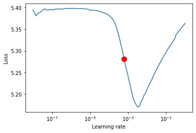
Finding good initial-learning rate using LRFinder algorithm
I use pytorch-lightning’s built-in LRFinder algorithm to find initial learning rate.
module = ImageEmbeddingModule(hparams)
t = pl.Trainer(gpus=1)
lr_finder = t.lr_find(module)
GPU available: True, used: True
TPU available: False, using: 0 TPU cores
CUDA_VISIBLE_DEVICES: [0]

   | Name  | Type            | Params
------------------------------------------
0 | model | ImageEmbedding  | 6 M
1 | loss  | ContrastiveLoss | 0
lr_finder.plot(show=False, suggest=True)
lr_finder.suggestion()
0.000630957344480193
I also use W&B Logging to keep track of my experiments:
from pytorch_lightning.loggers import WandbLogger
hparams = Namespace(
    lr=0.000630957344480193,
    epochs=10,
    batch_size=160,
    train_size=20000,
    validation_size=1000
)
module = ImageEmbeddingModule(hparams)
logger = WandbLogger(project="simclr-blogpost")
logger.watch(module, log="all", log_freq=50)
trainer = pl.Trainer(gpus=1, logger=logger)
trainer.fit(module)
| Name  | Type            | Params
------------------------------------------
0 | model | ImageEmbedding  | 6 M
1 | loss  | ContrastiveLoss | 0
After the training completes, embeddings are ready for usage for the downstream tasks.
Image classifier on top of SimCLR embeddings
Once the embeddings are trained, they can be used to train the classifier on top of them - either by fine tuning the whole network or by freezing the base network with embeddings and learning linear classifiers on top of it - I show the latter below.
Save the weights of neural network with embeddings
I save the whole network in a form on a checkpoint. Only the internal part of the network will be used later with the classifier (projection layers will be discarded).
checkpoint_file = "efficientnet-b0-stl10-embeddings.ckpt"
trainer.save_checkpoint(checkpoint_file)
trainer.logger.experiment.log_artifact(checkpoint_file, type="model")
Classifier module
Again, I define a custom module - this time it uses already existing embeddings and freezes the base model weights on demand. Note the SimCLRClassifier.embeddings are only the EfficientNet part of the whole network used before - the projection head is discarded.
class SimCLRClassifier(nn.Module):
    def __init__(self, n_classes, freeze_base, embeddings_model_path, hidden_size=512):
        super().__init__()

        base_model = ImageEmbeddingModule.load_from_checkpoint(embeddings_model_path).model

        self.embeddings = base_model.embedding

        if freeze_base:
            print("Freezing embeddings")
            for param in self.embeddings.parameters():
                param.requires_grad = False

        # Only linear projection on top of the embeddings should be enough
        self.classifier = nn.Linear(in_features=base_model.projection[0].in_features,
                      out_features=n_classes if n_classes > 2 else 1)


    def forward(self, X, *args):
        emb = self.embeddings(X)
        return self.classifier(emb)
Classifier training code
Classifier training code again uses PyTorch lightning, so I’m skipping in-depth explanation.
from torch import nn
from torch.optim.lr_scheduler import CosineAnnealingLR
class SimCLRClassifierModule(pl.LightningModule):
    def __init__(self, hparams):
        super().__init__()
        hparams = Namespace(**hparams) if isinstance(hparams, dict) else hparams
        self.hparams = hparams
        self.model = SimCLRClassifier(hparams.n_classes, hparams.freeze_base,
                                      hparams.embeddings_path,
                                      self.hparams.hidden_size)
        self.loss = nn.CrossEntropyLoss()

    def total_steps(self):
        return len(self.train_dataloader()) // self.hparams.epochs

    def preprocessing(seff):
        return transforms.Compose([
                transforms.ToTensor(),
                transforms.Normalize(mean=[0.485, 0.456, 0.406], std=[0.229, 0.224, 0.225]),
        ])

    def get_dataloader(self, split):
        return DataLoader(STL10(".", split=split, transform=self.preprocessing()),
                          batch_size=self.hparams.batch_size,
                          shuffle=split=="train",
                          num_workers=cpu_count(),
                         drop_last=False)

    def train_dataloader(self):
        return self.get_dataloader("train")

    def val_dataloader(self):
        return self.get_dataloader("test")

    def forward(self, X):
        return self.model(X)

    def step(self, batch, step_name = "train"):
        X, y = batch
        y_out = self.forward(X)
        loss = self.loss(y_out, y)
        loss_key = f"{step_name}_loss"
        tensorboard_logs = {loss_key: loss}

        return { ("loss" if step_name == "train" else loss_key): loss, 'log': tensorboard_logs,
                        "progress_bar": {loss_key: loss}}

    def training_step(self, batch, batch_idx):
        return self.step(batch, "train")

    def validation_step(self, batch, batch_idx):
        return self.step(batch, "val")

    def test_step(self, batch, batch_idx):
        return self.step(Batch, "test")

    def validation_end(self, outputs):
        if len(outputs) == 0:
            return {"val_loss": torch.tensor(0)}
        else:
            loss = torch.stack([x["val_loss"] for x in outputs]).mean()
            return {"val_loss": loss, "log": {"val_loss": loss}}

    def configure_optimizers(self):
        optimizer = RMSprop(self.model.parameters(), lr=self.hparams.lr)
        schedulers = [
            CosineAnnealingLR(optimizer, self.hparams.epochs)
        ] if self.hparams.epochs > 1 else []
        return [optimizer], schedulers
It’s worth mentioning here that training with a frozen base model gives a great performance boost during training as the gradients need to be calculated only for a single layer. Additionally, by utilizing good embeddings, only a few epochs are required to reach a good quality classifier with single linear projection.
hparams_cls = Namespace(
    lr=1e-3,
    epochs=5,
    batch_size=160,
    n_classes=10,
    freeze_base=True,
    embeddings_path="./efficientnet-b0-stl10-embeddings.ckpt",
    hidden_size=512
)
module = SimCLRClassifierModule(hparams_cls)
logger = WandbLogger(project="simclr-blogpost-classifier")
logger.watch(module, log="all", log_freq=10)
trainer = pl.Trainer(gpus=1, max_epochs=hparams_cls.epochs, logger=logger)
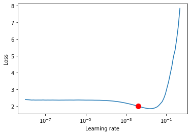
lr_find_cls = trainer.lr_find(module)
| Name  | Type             | Params
-------------------------------------------
0 | model | SimCLRClassifier | 4 M
1 | loss  | CrossEntropyLoss | 0
LR finder stopped early due to diverging loss.
lr_find_cls.plot(show=False, suggest=True)
lr_find_cls.suggestion()
0.003981071705534969
hparams_cls = Namespace(
    lr=0.003981071705534969,
    epochs=5,
    batch_size=160,
    n_classes=10,
    freeze_base=True,
    embeddings_path="./efficientnet-b0-stl10-embeddings.ckpt",
    hidden_size=512
)
module = SimCLRClassifierModule(hparams_cls)
trainer.fit(module)
| Name  | Type             | Params
-------------------------------------------
0 | model | SimCLRClassifier | 4 M
1 | loss  | CrossEntropyLoss | 0
Evaluation
Here I define a utility function for evaluating the model using the provided data loader. Note the transfer between GPU and CPU and storing all results in-memory might be not effective for large datasets!
from sklearn.metrics import classification_report
def evaluate(data_loader, module):
    with torch.no_grad():
        progress = ["/", "-", "\\", "|", "/", "-", "\\", "|"]
        module.eval().cuda()
        true_y, pred_y = [], []
        for i, batch_ in enumerate(data_loader):
            X, y = batch_
            print(progress[i % len(progress)], end="\r")
            y_pred = torch.argmax(module(X.cuda()), dim=1)
            true_y.extend(y.cpu())
            pred_y.extend(y_pred.cpu())
        print(classification_report(true_y, pred_y, digits=3))
        return true_y, pred_y
_ = evaluate(module.val_dataloader(), module)
                  precision    recall  f1-score   support

               0      0.856     0.864     0.860       800
               1      0.714     0.701     0.707       800
               2      0.903     0.919     0.911       800
               3      0.678     0.599     0.636       800
               4      0.665     0.746     0.703       800
               5      0.633     0.564     0.597       800
               6      0.729     0.781     0.754       800
               7      0.678     0.709     0.693       800
               8      0.868     0.910     0.888       800
               9      0.862     0.801     0.830       800

        accuracy                          0.759      8000
       macro avg      0.759     0.759     0.758      8000
    weighted avg      0.759     0.759     0.758      8000
Summary
I hope you find my explanation of the SimCLR framework useful. Feel free to ask anything, comment, play with the notebook and share this post with the ML community!
Additional links and resources
- SimCLR paper - arxiv.org/pdf/2002.05709.pdf
- EfficientNet paper - arxiv.org/abs/1905.11946
- this notebook on GitHub - link
- this notebook on Google Colab - link
Comments